How To Disable Automatic Update Of Links In Excel 2016

In Google Sheets, there is a wonderful function called IMPORTRANGE. It allows you lot to import and link a specific range of cells from one spreadsheet to some other. Excel is older and provides more than intense functional stuffing, so information technology should as well have the IMPORTRANGE office available, right? Read on to discover the answer to this and many other Excel IMPORTRANGE related questions.

Is in that location IMPORTRANGE in Excel?

There are many functions in Excel, such equally VLOOKUP Excel or SUMIF Excel. Nonetheless, at that place is no IMPORTRANGE function.

At the same time, Excel provides a similar to IMPORTRANGE functionality for linking a data range from a separate spreadsheet. This can be done either by copying and pasting a data range or by using a formula bar.

What is the Excel version of IMPORTRANGE?

In Excel Online, the IMPORTRANGE functionality is called WorkBook links.

In Excel desktop, information technology has no explicit proper name, merely is implemented via the Paste Link option.

The implementation of an Excel IMPORTRANGE equiv depends on the Excel app y'all employ (365/Online or desktop app). Let'south discuss each way separately.

How to use IMPORTRANGE equivalent for Excel desktop

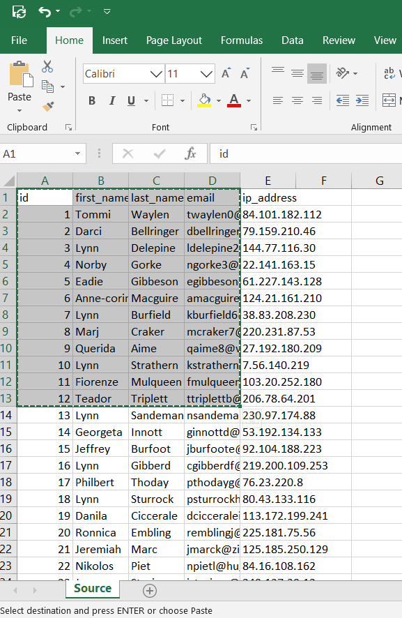
Open both a source and a destination Excel spreadsheet. Select a range of cells in the source spreadsheet and copy them: you can use either Ctrl+C or right click => Copy.

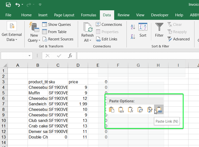
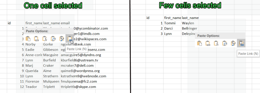
Go to your destination spreadsheet, select either one cell to import the entire range or a range of cells to only populate the selected cells. Then right-click and select Paste Link.

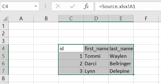
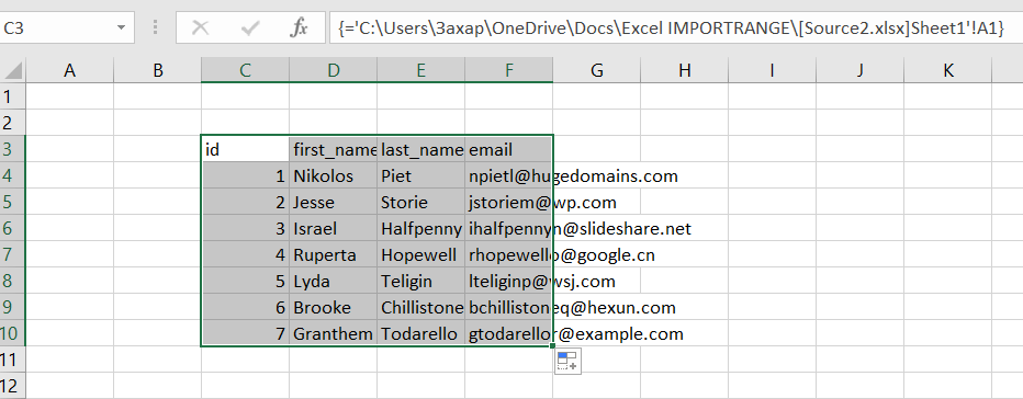
You can aggrandize the imported range by simply dragging the cross as follows:

Now if you change some values of the imported range in the source file, the values in the destination spreadsheet volition be updated as well.

This method works well if your source and destination spreadsheets are open up. When y'all need to import a range from an Excel workbook that is not open, use the formula bar method.

Excel IMPORTRANGE formula using the formula bar in desktop app

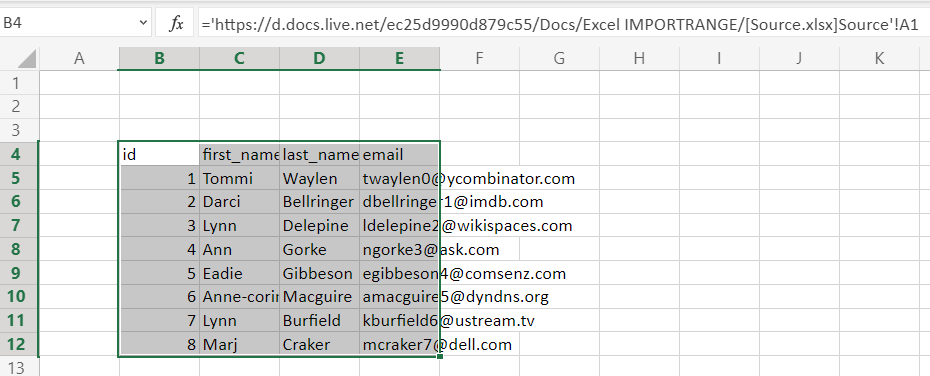
First of all, an important notation: If your source workbook simply has 1 worksheet with the same proper name equally the workbook, the imported range reference will look every bit follows in the formula bar:

                ={workbook-name}.xlsx!{first-cell}              

For case:

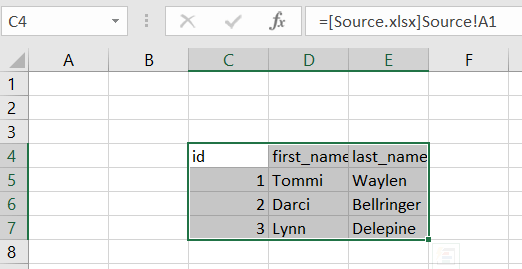
Nonetheless, if the names of the source workbook and worksheets differ, or the workbook has multiple worksheets, the imported range reference will look as follows in the formula bar:

                =[{workbook-name}.xlsx]{worksheet-name}!{first-jail cell}              

For instance:

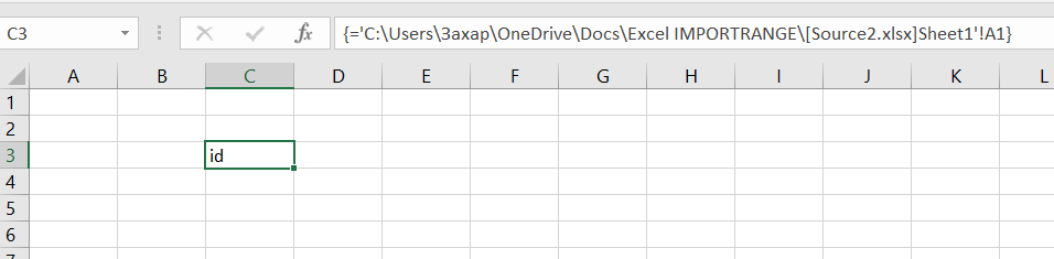
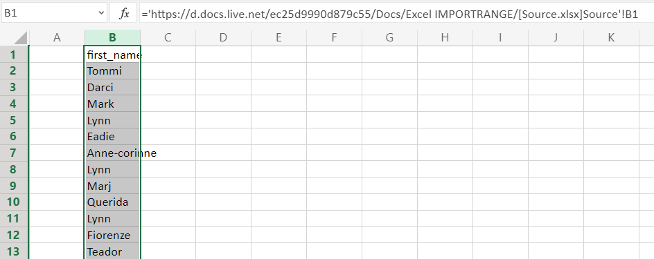
When you close the source workbook, the imported range reference transforms in the post-obit manner:

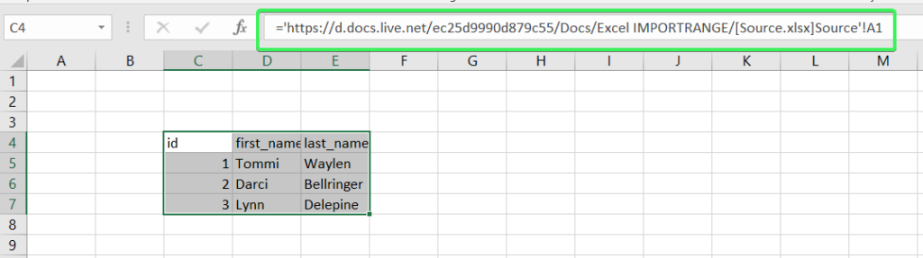
So, it's attached with a path to the file on your device. In our case, the path is to the OneDrive storage binder. However, yous can also meet the more regular paths like this one:

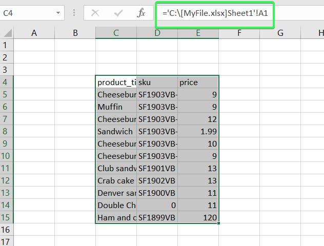
This is the average you can use to import data from any Excel file on your device:

                ='{path-to-file}/[{workbook-name}.xlsx]{worksheet-name}'!{first-jail cell}              

Note: yous can employ either slash or backslash depending on which type is used in the path to your file.

For instance, we need to import data from Sheet1 of a source file named Source2.xlsx stored in the OneDrive folder. In the example to a higher place, our reference to this binder looked every bit follows:

https://d.docs.live.net/ec25d9990d879c55/Docs/Excel IMPORTRANGE/

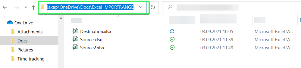
Just information technology's okay if y'all take a regular path, which you can find in the file explorer like this:

C:\Users\Захар\OneDrive\Docs\Excel IMPORTRANGE

Insert this path cord to the Excel IMPORTRANGE equivalent formula and add together other variables: {workbook-name}, {worksheet-name}, and {first-prison cell}. Here is what we've got:

='C:\Users\Захар\OneDrive\Docs\Excel IMPORTRANGE\[Source2]Sheet1'!A1

Select a cell, insert this formula to the formula bar and press Ctrl+Shift+Enter.

At present you can expand the range by dragging the cell vertically or horizontally.

If you desire to import an verbal range at in one case, specify the range instead of the outset cell in your formula. Then select the range in the destination sheet, insert the formula to the formula bar, and press Ctrl+Shift+Enter. Here is an instance:

='C:\Users\Захар\OneDrive\Docs\Excel IMPORTRANGE\[Source2]Sheet1'!A1:C10

Note: if yous select the number of cells greater than the number of cell in the range to import, you'll go #Due north/A for the cell across the range.

Workbook links – Excel IMPORTRANGE from dissimilar worksheet online

Now yous take agreement of how IMPORTRANGE functionality on Microsoft Excel desktop works. However, Excel Online, besides as Excel 365, has some differences in use. Permit'due south explore how Workbook Links works.

Open the files y'all already know, Source.xlsx and Destination.xlsx, in Excel Online. Select and copy a range in the source file, go to the destination file, select a cell, right-click and choose Link as a paste selection.

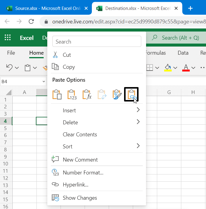
The cells will be populated with the values from the source spreadsheet.

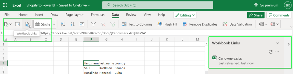
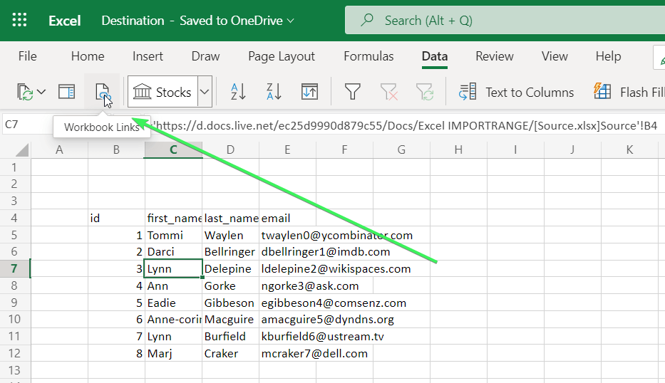
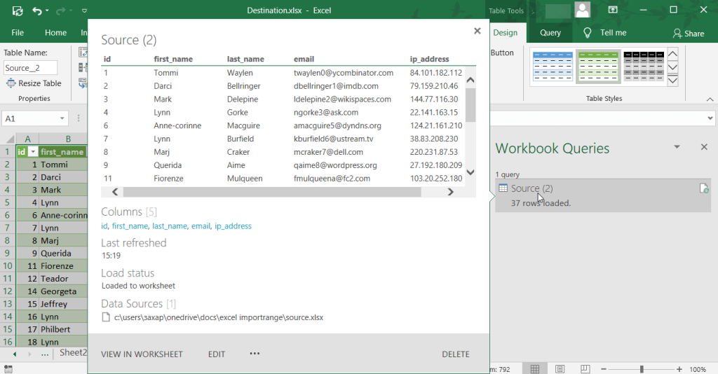
The main departure here is that the imported information won't be refreshed automatically until you lot enable this. To do this, go to the Data menu => Workbook Links.

On the popular-up panel on the right, click the 3 dots and bank check the Refresh automatically checkbox for the linked workbook.

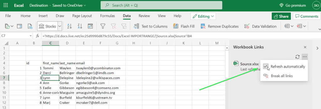
Now the imported range will be refreshed automatically every 5 minutes to brandish any change in the source range.

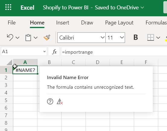
Excel Workbook Links does not piece of work

Nosotros tried to import a range from a file stored in some other folder, and here is the result:

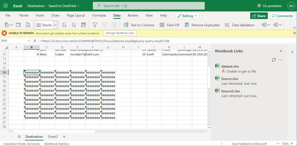
Nosotros referenced a thread on the MS Office forum regarding the aforementioned upshot, but nosotros've notwithstanding had no luck in resolving it. The only method that worked was to put the source and destination workbooks in the aforementioned folder.

With this in mind, it'due south good to have a failsafe alternative to link Excel to Excel. And there is 1 – Coupler.io.

IMPORTRANGE and Workbook Links alternative for Excel

Coupler.io is a tool for importing information from apps and sources to Excel, Google Sheets, or BigQuery. For example, you lot can export raw information from Pipedrive or HubSpot and load it to your workbook stored on OneDrive. The main feature is that you can schedule automatic data refresh for your information.

In our instance, we need to synchronize 2 Excel spreadsheets, and this is easily doable. Bank check out the bachelor Excel integrations.

Sign up to Coupler.io, click "Add new importer", name it any you want, and complete these 3 steps:

• Ready source
• Fix destination
• Fix schedule

Set up source

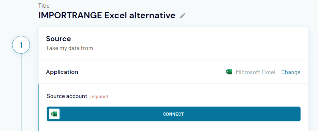
• Select Microsoft Excel every bit a source application.

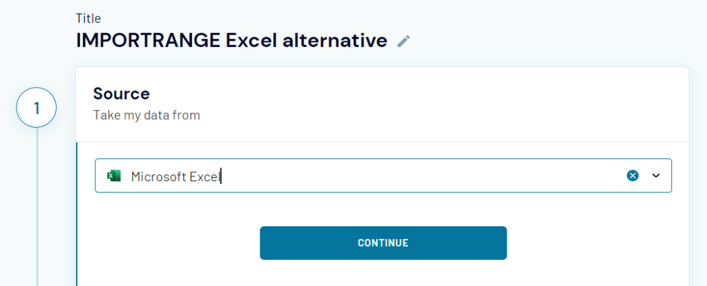
• Connect your Microsoft account.

• Select a source workbook from your OneDrive folder and specify a worksheet or multiple worksheets.

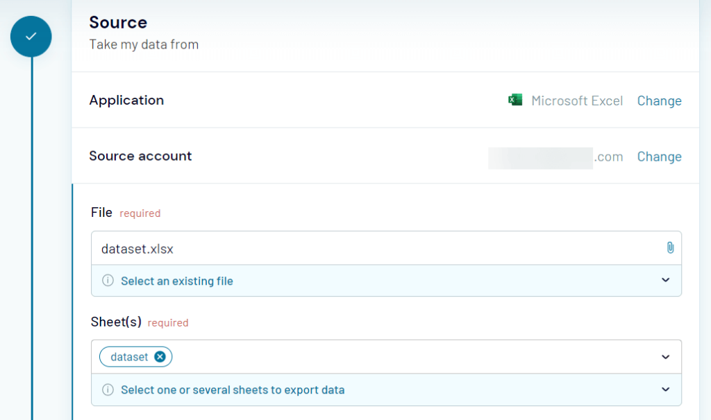
Note: Selecting multiple sheets tin can be used if you want to concatenate data from multiple sheets into ane.

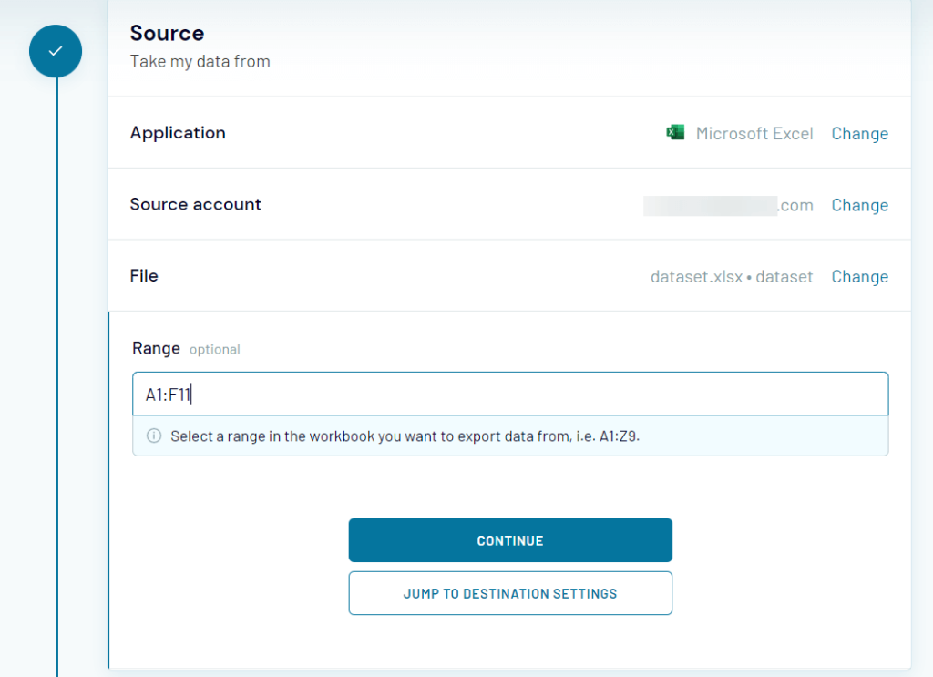
• Specify a range to import. Subsequently that you can get to the destination setup.

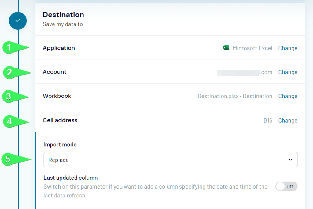
Set up destination

The flow is by and large the same:

• Select Microsoft Excel as a destination app
• Connect your Microsoft account or select an existing 1
• Select a destination workbook from your OneDrive folder and specify a worksheet.
• Specify the first cell to load data to.
• Select the import style:
  • Supercede – to replace all data
  • Append – to append newly imported records under the previously imported ones

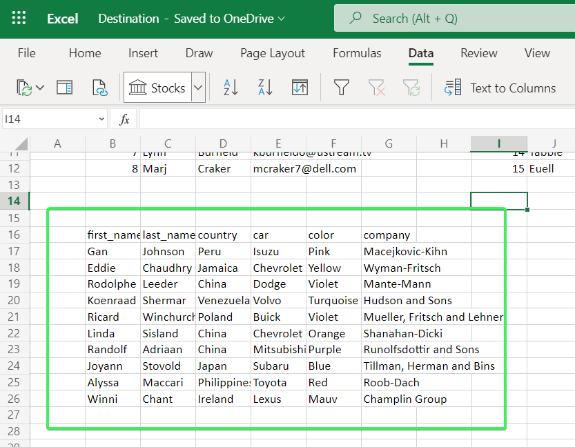
Click "Save and Run" to import a range to your destination spreadsheet. Voila!

Expect, we've talked about iii steps, correct?

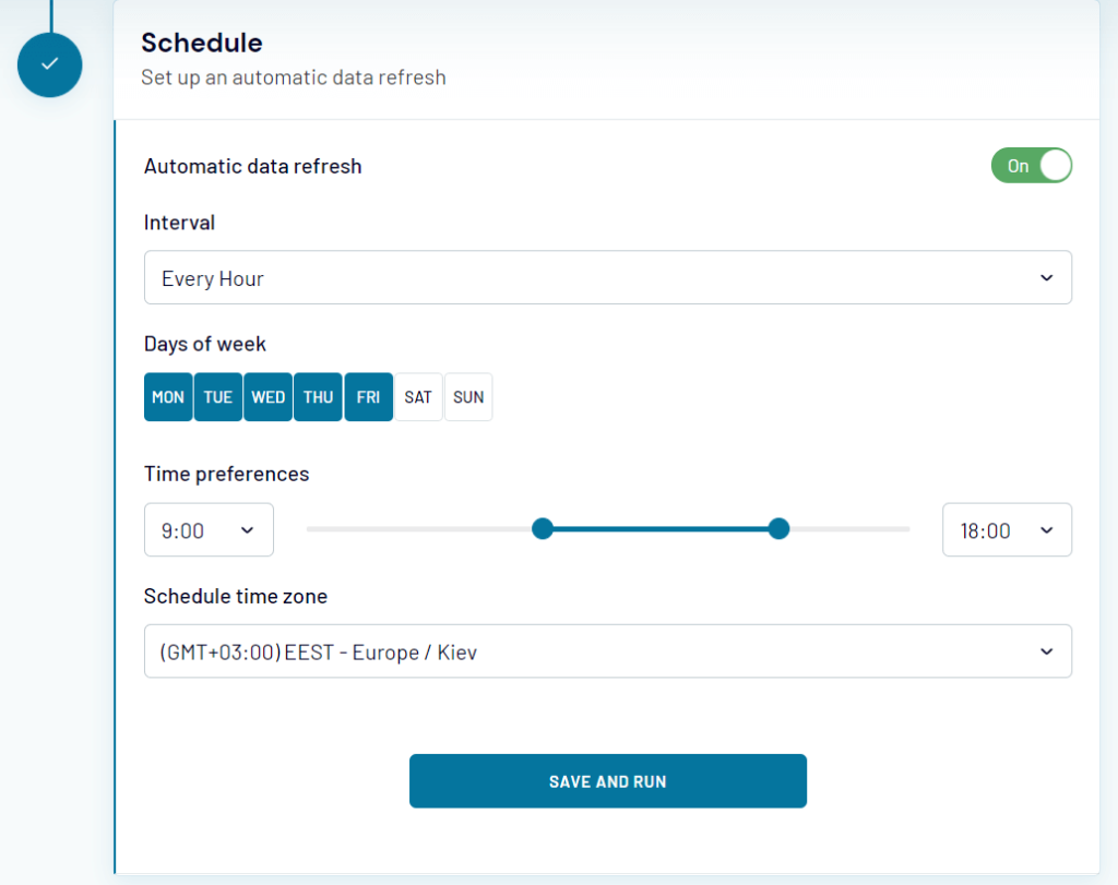
Set up schedule

Coupler.io allows you lot to automate import of data on a custom frequency – for example, every hour or every Tuesday. To do this, toggle on the Automatic data refresh and configure the schedule for your data import.

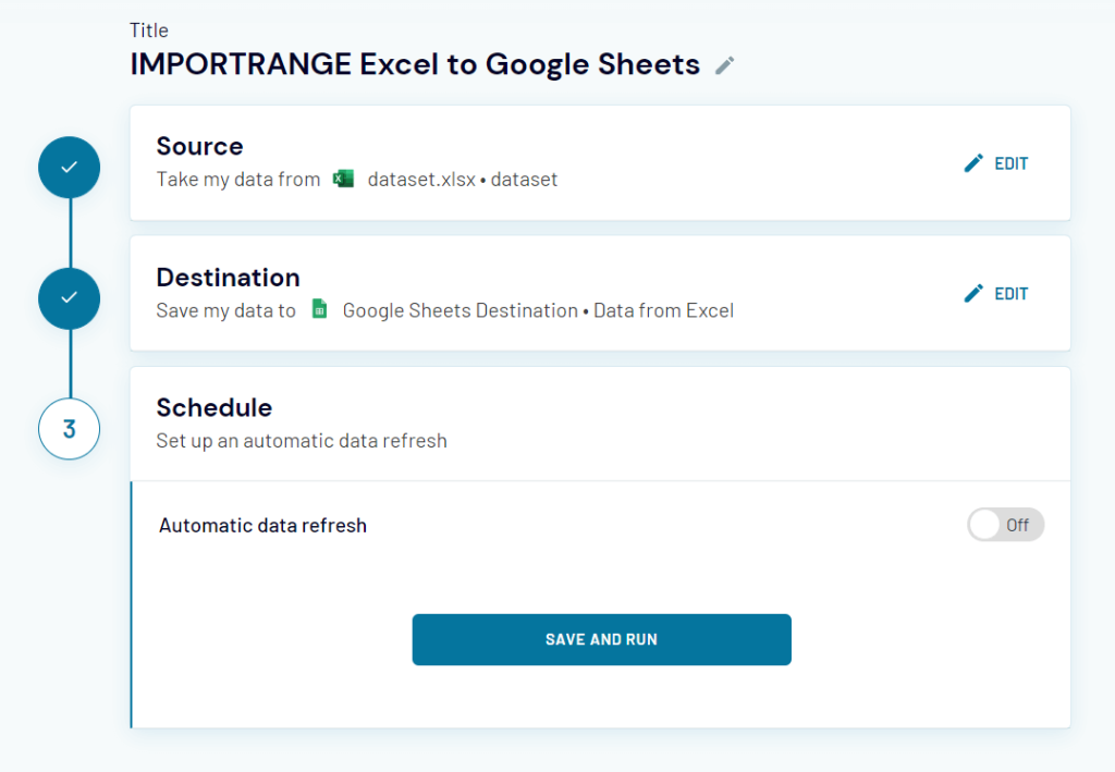
IMPORTRANGE from Excel to Google Sheets and vice versa

The real IMPORTRANGE function only connects Google Sheets documents. IMPORTRANGE in Excel, Workbook Links, simply connects Excel files. With Coupler.io, yous can mix those functionalities and synchronize data between an Excel workbook and a Google spreadsheet.

For example, to import a range from an Excel spreadsheet to Google Sheets, you need to cull Excel as a source app and select the file to get data from. Equally a destination app, choose Google Sheets, and select the file to load data to. Hither is what it should look similar:

Excel IMPORTRANGE FAQs

Two most pop spreadsheet apps, Google Sheets and Excel, accept a big influence on each other'south progress. IMPORTRANGE is a case in point, because it's a Google Sheets function that is not available in Excel. Nevertheless, many users keep using the term Excel IMPORTRANGE to proper name Workbook Links…or they just dream well-nigh a day when the Microsoft team releases this function. 🙂 Anyhow, we nerveless a few questions associated with this and hope you lot'll observe it useful.

Excel IMPORTRANGE function for a whole column

Everything works as usual. To import an unabridged column from one workbook to another, merely select the column (click the column index letter of the alphabet), copy it, and paste as link into the destination workbook.

How to use Excel IMPORTRANGE to get data with formatting?

IMPORTRANGE in Google Sheets, Workbook Links in Excel, likewise equally Coupler.io, allow you to just import raw information without formatting.

Can I utilise Excel IMPORTRANGE with CONCATENATE?

In Google Sheets, yous tin can nest IMPORTRANGE with CONCATENATE, QUERY, and many other functions. For example, bank check out our IMPORTRANGE+QUERY tutorial.

Nevertheless, in Excel, there is no IMPORTRANGE function, and so it's incommunicable to do.

Excel IMPORTRANGE to import cells with text only

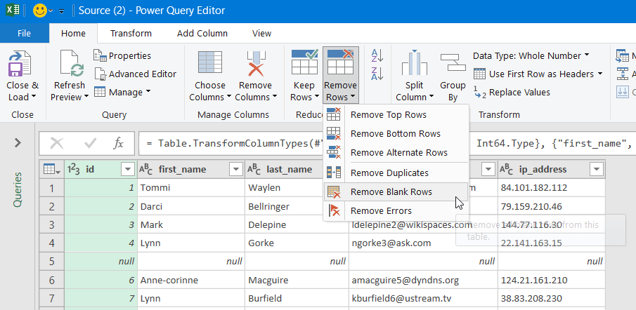
Unfortunately, Workbook Links does not allow you set weather for the ranges you import. Nonetheless, you can use the Excel Power Query to do the job. For example, our information gear up that we need to import contains empty rows:

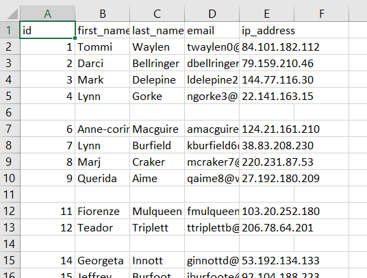
We can set a condition to ignore them for our import.

• Become to the Information menu => New Query => From File => From Workbook

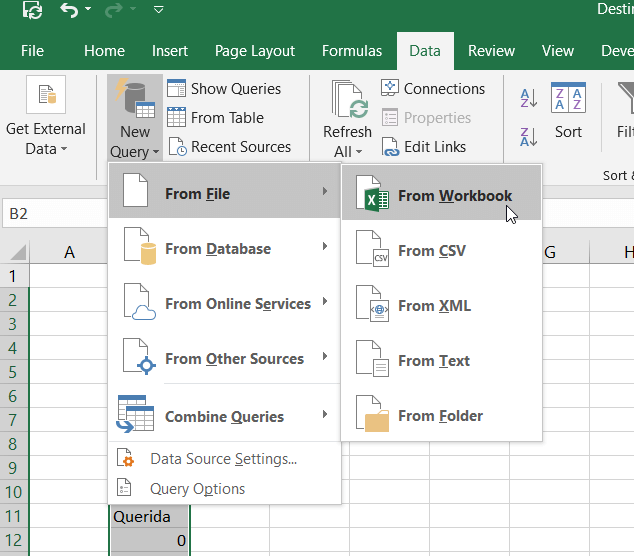
• Select your source workbook. In the Navigation window, select a sheet and click "Transform Data".

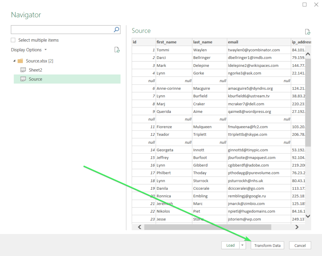
• This will bring you to the Power Query Editor, where y'all tin add or remove columns/rows, change data types, split columns, group values by columns, and perform other sorts of data manipulation. What we need is to remove blank rows. In that location is a dedicated button for this on the ribbon menu: Remove Rows => Remove Blank Rows.

• All bare rows have been removed. Now you can Close & Load your information range. Click the respective push.

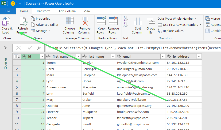
• Welcome your data range into your sheet. At present the source sheet is connected to your destination sheet, and the queried data range volition be refreshed automatically every 5 minutes, or you can do this manually.

IMPORTRANGE, Workbook Links, or Coupler.io

Who's going to win this race? Only Coupler.io is designed for both Excel and Google Sheets users and provides them with a scheduled data refresh, support for multiple sources and destinations, and many other cool features.

IMPORTRANGE is only available for Google Sheets users. It'south a good office, although it is known for its errors, which we've covered in Why IMPORTRANGE Is Not Working: Errors and Fixes.

Workbook Links, looks a bit plain and straightforward compared to its competitors. The keyword "excel importrange" is highly requested in Google search results, which means that Excel users need this function instead of WL. Ugly truth.

So, make your selection for importing data and proficient luck with it!

Dorsum to Blog

Admission your information

in a simple format for free!

Commencement Free

Source: https://blog.coupler.io/importrange-excel/

Posted by: holtthea1980.blogspot.com

Share this post